In Part 1, I created a neural network that learns to represent a 2D image by mapping pixel coordinates to RGB colors. I built a multilayer perceptron (MLP) that takes x,y pixel positions as input, applies sinusoidal positional encoding to transform the 2D coordinates into a 42-dimensional vector (using L=10 frequency levels), and processes this through several linear layers with ReLU activations to output RGB values. For training, I implemented a dataloader that randomly samples batches of pixels since processing all pixels at once would be memory-intensive. I used MSE loss with Adam optimizer (learning rate 1e-2) and tracked the network's performance using PSNR (Peak Signal-to-Noise Ratio) as my metric.
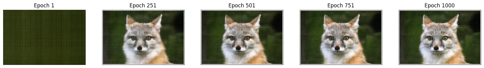
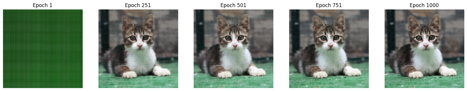
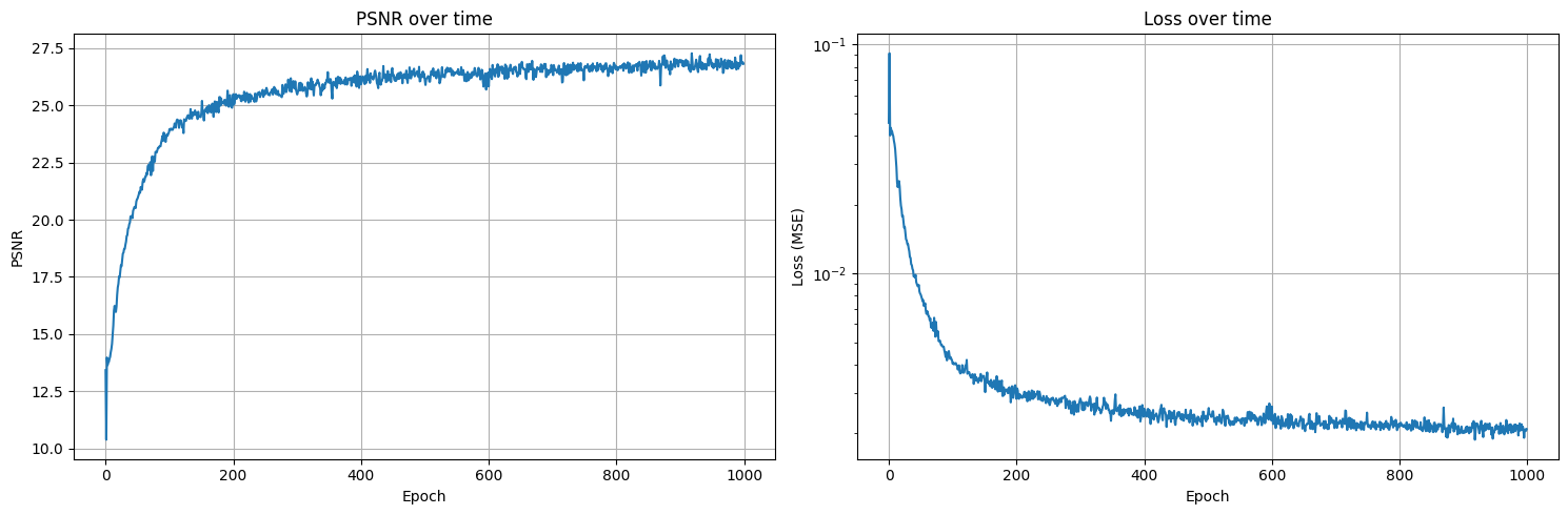
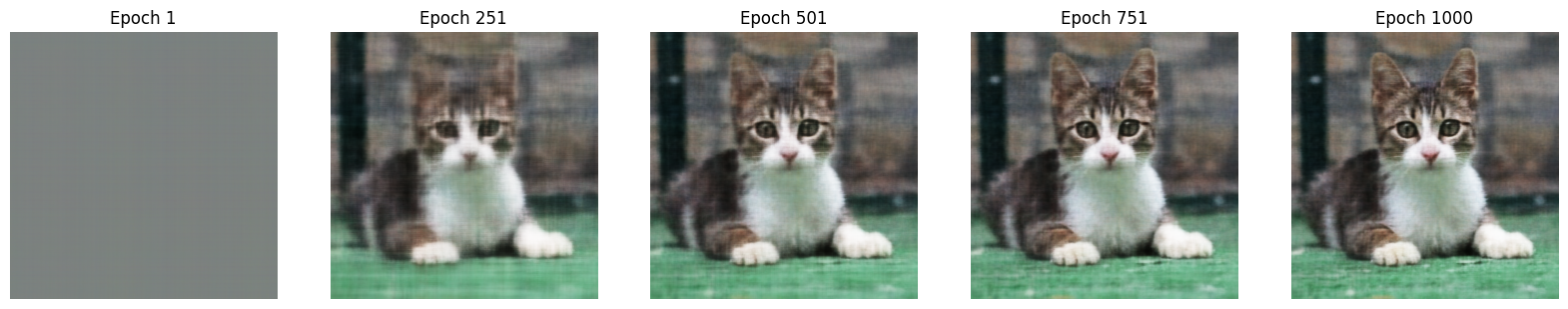
My network architecture consisted of 4 linear layers (256 channels each) with ReLU activations, followed by a final layer outputting RGB values. I tested it on two different images - a fox photograph and a cat photograph. The training visualizations show interesting progression: starting from solid-colored approximations at Epoch 1, by Epoch 251 both images show clear subject definition, and by Epoch 501-1000 the network captures fine details like fur textures and facial features. I conducted hyperparameter tuning experiments, varying the network depth, width, and positional encoding frequencies. The PSNR curves for both images show rapid initial improvement followed by gradual refinement, with the network achieving high-quality reconstructions by Epoch 1000. The cat image's hyperparameter tuning led to interesting changes: the convergence process due to the learning rate being increased and L being modified was slower, and as a result, the first plot shows significantly more noise than the result with the default parameters without tuning. The parameters were 1) num_epochs=1000, batch_size=10000, lr=1e-2, L=10, layers=4 and 2) num_epochs=1000, batch_size=10000, lr=1e-3, L=5, layers=4
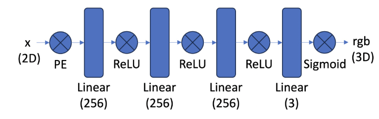
Nerf 2D Architecture
Optimizing Process #1
PSNR and Training Plots
Optimizing Process #2
After Hyperparameter Tuning #2
In Part 2, I expanded my neural field implementation to handle 3D space representation using a technique called Neural Radiance Fields (NeRF). Instead of working with a single 2D image, I now worked with multiple calibrated images of a Lego scene taken from different viewpoints. The dataset included 100 training images, 10 validation images, and 60 test camera positions for novel view synthesis, all at 200x200 resolution. Each image came with its corresponding camera-to-world transformation matrix and focal length. The visualization shows the camera positions distributed around the scene, with training cameras in black, validation in red, and test views in green, illustrating how the images capture the scene from multiple angles to enable 3D reconstruction.
In Part 2.1, I worked on implementing the camera and ray mathematics that form the foundation of NeRF. I developed functions to handle coordinate transformations between different spaces: world, camera, and pixel coordinates. I implemented the transform function that converts points between camera and world space using camera-to-world transformation matrices, and created functions to handle pixel-to-camera coordinate conversions using the camera's intrinsic matrix K (which depends on focal length and principal point). Finally, I built a ray generation system that creates rays for each pixel by calculating their origins (camera positions) and directions (normalized vectors from camera through pixels). These rays are crucial for the volume rendering process that NeRF uses to generate novel views.
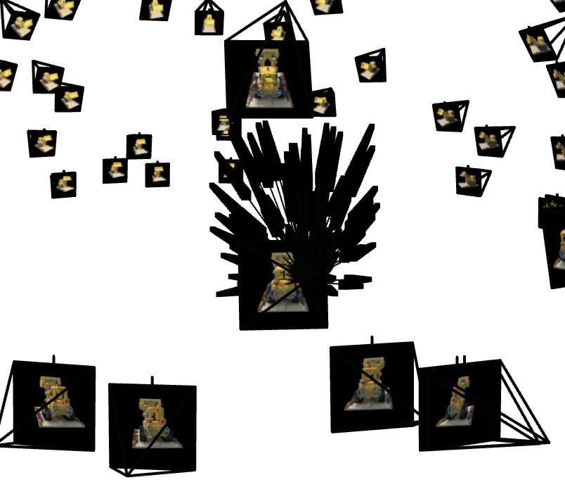
In Part 2.2, I implemented the sampling strategies needed for NeRF. The first part involved sampling rays from the training images - I could either randomly sample N rays from each image or flatten all pixels and sample globally. Building on Part 1's image sampling, I added a +0.5 offset to center the sampling grid on pixels. For each sampled ray, I then implemented point sampling along its length between near=2.0 and far=6.0 planes. To prevent overfitting, I added small random perturbations to these sample points during training. These sample points along each ray would later be used by the NeRF network to predict color and density values. I set the number of samples per ray to either 32 or 64 for this project.
In Part 2.3, I developed a comprehensive dataloader that integrates all the previous components needed for training NeRF with multiple views. The dataloader's main job is to randomly sample pixels from the training images and convert them into rays using the camera parameters. This is more complex than Part 1's simple 2D sampling because now we need to handle camera intrinsics (focal length, principal point) and extrinsics (rotation and translation matrices) to generate proper rays. For each batch, the dataloader returns ray origins, ray directions, and the corresponding pixel colors from the training images.
To help debug and verify my implementation, I created visualization code using the Viser library. This generates an interactive 3D view showing the camera frustums (the pyramidal viewing volume of each camera), the sampled rays, and the 3D sample points along those rays. The visualization was crucial for ensuring everything was working correctly - I could visually confirm that rays were being generated in the right directions and that sample points were properly distributed in 3D space. I also implemented checks to verify that rays stay within the camera frustum and added assertions to test that my pixel sampling matched the ground truth values. This careful verification process helped catch and fix several subtle bugs in the coordinate transformations and sampling logic.
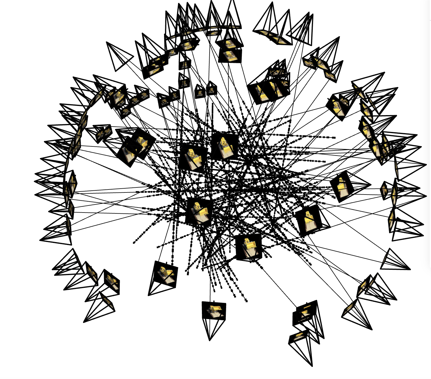
1st Visual
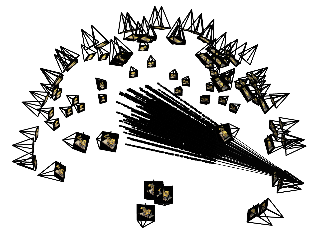
2nd Visual Rays through Image
2nd Visual Angle 2
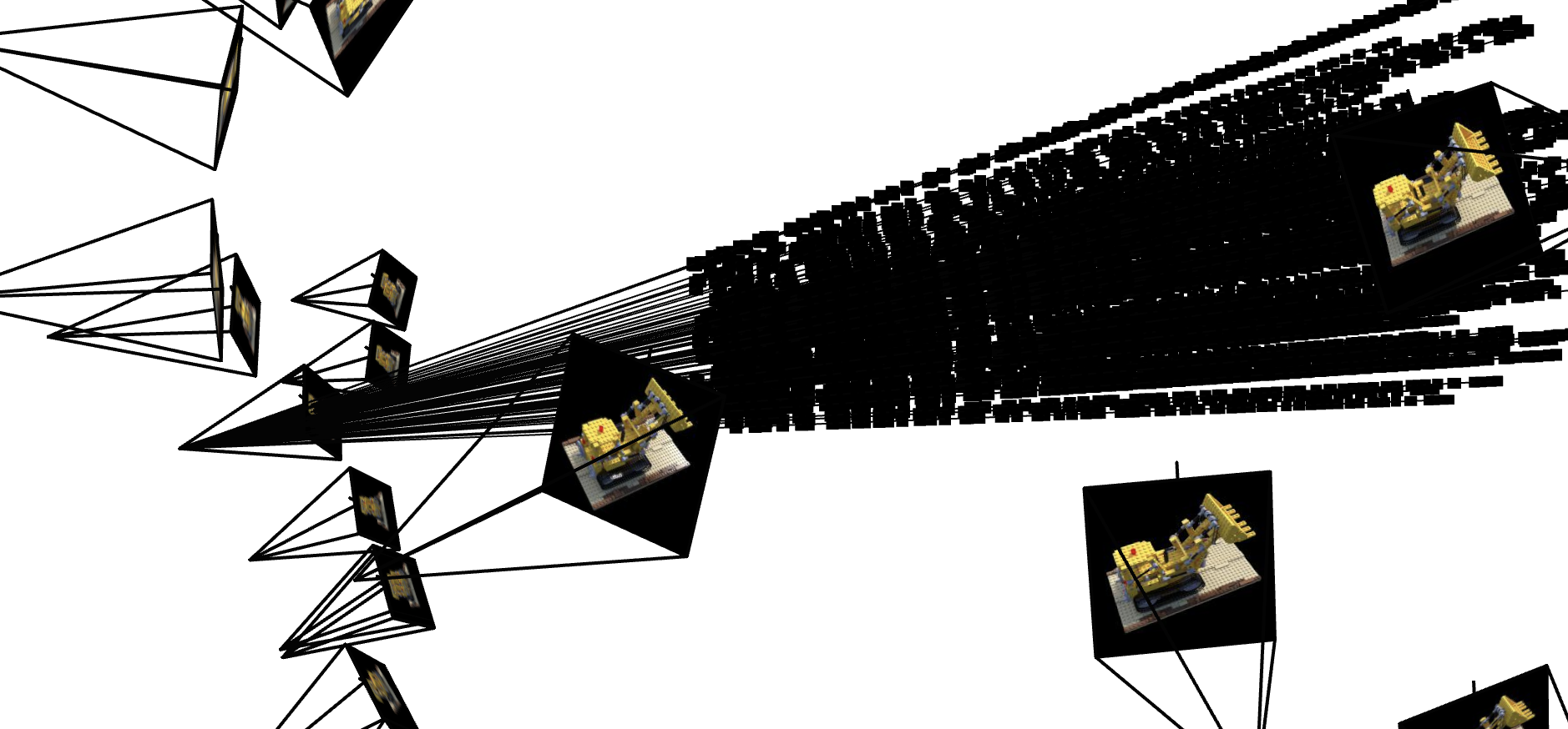
2nd Visual Angle 3
In Part 2.4, I implemented the core Neural Radiance Field (NeRF) network architecture, which builds upon the MLP from Part 1 but with several key modifications for handling 3D scenes. The network takes 3D world coordinates and view directions as input, applying positional encoding (though with fewer frequency levels L=4 compared to L=10 for coordinates) to both. The architecture is significantly deeper than in Part 1, reflecting the more complex task of learning a 3D representation. A crucial design element is that the network outputs both density (opacity) and color for each 3D point - density is view-independent and uses ReLU activation to ensure positive values, while color is view-dependent and uses sigmoid activation to stay within [0,1]. The network also employs a skip connection by concatenating the encoded input coordinates halfway through, which helps prevent the network from "forgetting" spatial information as it processes through many layers.
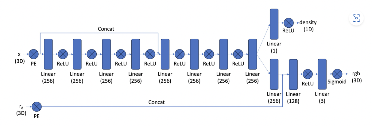
Nerf 3D Architecture
In Part 2.5, I implemented the volume rendering component of NeRF, which is crucial for generating novel views from the learned 3D representation. The process follows the physics of light transport, where we compute how light accumulates along each ray by considering both color and opacity (density) at each sample point. The mathematical formulation uses an integral equation that accounts for both the color contribution at each point and the transmittance (probability of light reaching that point without being blocked). Since we can't compute this integral analytically, I implemented a discrete approximation that steps along each ray, accumulating color contributions weighted by their transmittance values. The implementation needed to be done in PyTorch to enable backpropagation during training. I validated my implementation against a provided test case that checks if the rendered colors match expected values within a small tolerance, ensuring the mathematical correctness of the volume rendering computation.
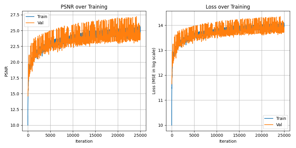
Training and PSNR Curves
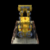
Rotation .gif, PSNR 25.5, 25000 Iterations, 1e-3 Learning Rate, 7500 Batch Size
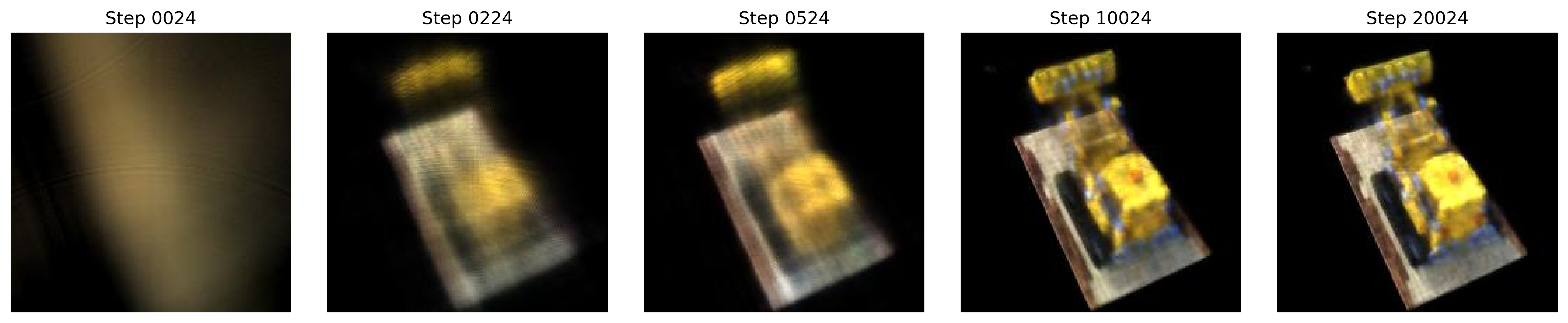
Training Progression from one camera view
Rays and samples at a single training step
In this B&W, I modified the NeRF's volume rendering implementation to support custom background colors instead of the default black background. This involved updating the rendering equation to properly handle accumulated transmittance. When a ray doesn't hit any dense objects (transmittance remains high), it should show the background color instead of black. I achieved this by adding the background color contribution term (1 - accumulated_opacity) * background_color to the volume rendering equation, where accumulated_opacity represents how much of the ray's visibility has been blocked by the scene. This allows the background color to show through in transparent regions while maintaining proper compositing with the scene geometry. The final rendered video of the Lego scene now appears with my chosen background color, creating a more visually appealing result while maintaining physically accurate light transport simulation.
Rotation .gif w modified background color
In this project, I dove deep into implementing Neural Radiance Fields (NeRF) from scratch, progressing from a simple 2D neural representation of images to a full 3D scene reconstruction system. What fascinated me most was understanding how NeRF combines several elegant ideas - positional encoding for capturing high-frequency details, volume rendering for realistic view synthesis, and clever sampling strategies along rays - to achieve such impressive 3D reconstructions from just a set of 2D images.